Newton's law in Cartesian and Cylindrical coordinates

• Newton's law: $\myv F=m\myv a$. This is what we'll call the "Equation of Motion".
• Newton's law in Cartesian coordinates.
• Finding a solution:
  • Integrating the equation of motion
  • Method of separation of variables
  • Application: motion in a gravitational field.
• Newton's law in polar (cylindrical) coordinates
• Application: skateboarder on a half-pipe

Newton's laws in Cartesian coordinates

...have a very simple form, since the unit vectors do not change with position. The position $\myv{r}$ of a particle is $$\myv{r} = x \uv{x} + y \uv{y} + z \uv{z}$$ $$\myv{v} = \dot{\myv{r}} = \frac{d}{dt} \myv{r} = \dot{x} \uv{x} + \dot{y} \uv{y} + \dot{z} \uv{z}$$ $$\myv{F} = m \myv{a} = m \ddot{\myv{r}} = m \ddot{x} \uv{x} + m \ddot{y} \uv{y} + m \ddot{z} \uv{z}$$

Integrating, to solve the equations of motion

Vasily Koloda - Unsplash

Projectile motion

...using an example you'll (probably!) remember from General physics: Two-d motion in a gravitational field. Newton's equation is: $$\begineq \myv F &= m\myv a\\ -mg \uv z &= m(\ddot x \uv x + \ddot z \uv z)\\ -g\uv z&=\ddot x \uv x + \ddot z \uv z \endeq $$

In order for the vector quantities on the left and right to be equal, the $x$ components must be equal and separately, the $z$ components must be equal. This leads to two differential equations: $$\uv x\text{ components: } 0 = \ddot x.$$ $$\uv z\text{ components: } -g = \ddot z.$$

Horizontal, $x$- motion

Taking the $x$ equation first, we have: $$\ddot x = \dot v_x=\frac{dv_x}{dt}=0.$$ We'll use the Method of separation of variables to solve this. We'll "take apart" $\frac{dv_x}{dt}$ into differentials, and re-arrange the parts, trying to get all the pieces that involve $v_x$ on one side of an equation, and all the pieces that involve $t$ on the other: $$dv_x=0\,dt.$$ Now, integrate both sides: $$\begineq \int_{v_{x}(t=0)}^{v_x(t)}\,dv_x' &= \int_{t'=0}^{t'=t} 0\,dt' \\ v_x(t)-v_x(0) &= 0. \endeq $$

The solution is $v_x(t)= v_x(0)\equiv v_{x0}$ (constant speed).

Now, repeating this process for $v_x(t)=\frac{dx}{dt} = v_{x0}$, separating the variables and setting up the integrals gives... $$\begineq \int_{x'=x(t=0)}^{x(t)}dx' =& \int_{t'=0}^{t}v_{x0}\,dt' =v_{x0}\int_{t'=0}^{t'=t}1\,dt'\\ x(t)-x_0 =& v_{x0}*(t-0) \endeq $$ Or $x(t)=x_0 + v_{x0}t$.

Vertical, $z$- motion

The equation for the vertical component of motion was $-g = \ddot z$, which can be written as $-g = \dot v_z=\frac{d v_z}{dt}$.

Separating variables and integrating once, $$\begin{align*} dv_z=&-g\,dt\\ \int_{v_z(0)}^{v_z(t)}dv'_z=&\int_0^t -g\,dt'\\ v_z(t)-v_{z0}=&-gt. \end{align*}$$ and rearranging gives $$v_z(t)=v_{z0}-gt.$$

Writing $v_z=\frac{dz}{dt}$, we repeat the process, separating variables and integrating again... $$\begin{align*} dz &= (v_{z0}-gt)\, dt\\ \int_{z_0}^{z(t)} dz' &=\int_0^t (v_{z0}-gt')\, dt'\\ z(t)-z_0 &=v_{z0}t -\frac12 g t^2 \end{align*}$$ And re-arranging just a bit, finally:

$$\begin{equation}z(t)=z_0+v_{z0}t-\frac12 g t^2.\end{equation}$$

Cylindrical coordinates

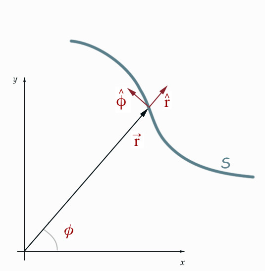Imagine that a particle follows a trajectory shown as $S$. In two dimensions the polar coordinates $r(t)$ and $\phi(t)$ are related to $x(t)$ and $y(t)$ as shown: $$x= r \cos \phi;\ \ y = r \sin \phi $$ $$r = \sqrt{ x^2 + y^2};\ \ \phi = \arctan ( y/x ) $$

Motion in cylindrical coordinates

Now imagine a particle moving along the path $S$ as shown. To express the velocity in terms of polar coordinates, our first approach will be to decompose the general change in position $\Delta \myv{r}$ into radial (along $\uv{r}$) and angular (along $\uv{\phi}$) components. From the diagram:

$$\myv r(t+\Delta t)-\myv r(t)\equiv\Delta \myv{r} \approx \Delta r \,\uv{r} + r \Delta \phi \,\uv{\phi}$$

Dividing this expression by $\Delta t$ and taking the limit should formally give us the derivative... $ \frac{\Delta \myv{r}}{\Delta t} = \frac{\Delta r}{\Delta t} \uv{r} + r \frac{\Delta \phi}{\Delta t} \uv{\phi} \rightarrow$...

$$\bnum \dot{\myv{r}} =\dot{r} \uv{r} + r \dot{\phi} \uv{\phi}. \enum$$

Alternative approach: Using the PRODUCT rule / Changes in the unit vectors

A slightly different way of approaching the problem is to use the changes in the unit vectors.

The length of the unit vectors (1 unit!) never changes with position/time, but their orientation changes.

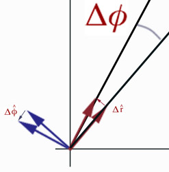During a time interval of $\Delta t$, a change of $\Delta r$ occurs in the $\uv r$ unit vector. But this does not change the magnitude (1) or the direction of this unit vector at all. So, the changes in the unit vectors depend only on the change of $\Delta \phi$ (during a time interval of $\Delta t$): $$\Delta \uv{r} \approx \Delta \phi \uv{\phi};\ \Delta \uv{\phi} \approx - \Delta \phi \uv{r}$$

Now we divide each expression by $\Delta t$, and take the limit of small time intervals:

$$\bnum\frac{d \uv{r}}{dt} = \frac{d \phi}{dt} \uv{\phi};\ \frac{d \uv{\phi}}{dt} = - \frac{d \phi}{dt} \uv{r}.\enum$$

Now, to find $v$, we need to find the rate of change of the position vector, which can be written as $\myv{r} = r \uv{r}$. Using the PRODUCT rule: $$\begineq \myv{v} =& \frac{d\myv r}{dt}= \frac{d}{dt} (r \uv{r}) \\ =& \frac{dr}{dt} \uv{r} + r \frac{d \uv{r}}{dt}\\ =& \dot{r} \uv{r} +r \dot{\phi} \uv{\phi} \endeq$$

And, since $\myv v\equiv \dot{\myv r}$, we get the same expression as above:

$$\bnum \dot{\myv{r}} =\dot{r} \uv{r} + r \dot{\phi} \uv{\phi}. \enum$$

Now, we can apply the product rule to this expression for the velocity, and we'll have the acceleration: $$\begineqnum \myv{a} =& \frac{d}{dt} \myv{v} = \frac{d}{dt} (\dot{r} \uv{r}+r\dot{\phi}\uv{\phi})\nonumber\\ =& \ddot{r} \uv{r} + \dot{r} \frac{d \uv{r}}{dt} + \dot{r} \dot{\phi} \uv{\phi} + r \ddot{\phi} \uv{\phi} + r \dot{\phi} \frac{d \uv{\phi}}{dt}\nonumber\\ =& \ddot{r} \uv{r} + \dot{r} \dot{\phi} \uv{\phi} + \dot{r} \dot{\phi} \uv{\phi} + r \ddot{\phi} \uv{\phi} - r \dot{\phi} \dot{\phi} \uv{r} \nonumber\\ \color{red}{\myv a}=& \color{red}{(\ddot{r} -r \dot{\phi}^2) \uv{r} + (2\dot{r} \dot{\phi} + r\ddot{\phi}) \uv{\phi} } \endeqnum $$

Example 1.2 / Problem 1.50 - Skateboard on a half-pipe

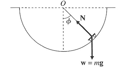A (frictionless) skateboard slides on a half-pipe of radius $R$. Our equation of motion is $\myv{F} = m \myv{a} = m[(\ddot{r} -r \dot{\phi}^2) \uv{r} + (2 \dot{r}\dot{\phi} + r\ddot{\phi}) \uv{\phi} ]$

But, it looks like $r=R$ is an unchanging constant ($\dot{r} = 0$). The $\uv r$ component will give us the changing force normal to the skateboard, but will not change $r=R$.

So, let's find the motion of $\phi(t)$. Consider the component of this equation in the $\uv{\phi}$ direction. Taking $\phi=0$ at the bottom of the half-pipe, $F_{\phi} = -mg \sin \phi = m R \ddot{\phi} $, then we have: $$-\frac{g}{R} \sin \phi = \ddot{\phi}$$

This is a non-linear differential equation, and there is no analytical solution. We will eventually use CoCalc to get a numerical solution to this differential equation and graph it.

But, we can still come up with an approximate solution: For small angles (and with angles as always in radians, $$\sin \phi \approx \phi.$$

PMR #1 - Graph $g(\phi)=\sin(\phi)$ and $f(\phi)=\phi$. (You can probably do this quicker on desmos.) At approximately what angle (radians) does the difference $|f(\phi)-g(\phi)|$ exceed 10% of $\phi$? What is that angle in degrees?

The equation of motion for such "small" differences is: $$-\frac{g}{R} \phi \approx \ddot{\phi}$$

Sagemath: solving differential equation

"Solving" means finding the function, $x(t)$, which satisfies:

• The equation of motion: usually a 2nd order differential equation of time, $t$,
• subject to a set of initial conditions. For example, you might have the initial position and velocity of a particle.

3 functions in Sagemath

• desolve(...): Solves a differential equation exactly / symbolically / analytically.
• desolve_system(...): Solves a system of differential equations exactly / symbolically / analytically.
• desolve_system_rk4(...): Solves a system of differential equation numerically (using the Runge-Kutta 4th order approximation).

Sagemath's numerical integration functions will solve a handful of 2nd order differential equation. It will solve our "simplified" Diff Eq for the skateboarder, but not the *exact* equation of motion.

Sagemath's more general way of solving differential equation is to solve systems of first order differential equation. And you can convert most second- and higher-order DiffEqs to systems.

See Handouts/halfpipe.../Skateboard-DiffEq.ipynb on CoCalc.

Systems of differential equation

If you can write a set of first order equations for $N$ variables, $x_1(t)$, $x_2(t)$,....$x_N(t)$ in the form: $$\begineq \dot{x}_1 =&f(x_1,x_2,...x_N)\\ \dot{x}_2 =&g(x_1,x_2,...x_N)\\ ...\\ \dot{x}_N =&z(x_1,x_2,...x_N)\\ \endeq $$ then Sagemath can usually solve the system. If you write these equations in terms of a single equation for an $N$-element column vector: $$\begincv \dot{x}_1 \\ \dot{x}_2 \\ ...\\ \dot{x}_N \endcv = \begincv f\\ g\\ ...\\ z \endcv $$ The right-hand side of the equation above are the elements of a list, which is the input to desolve_system... and the output is a list of functions which represents $x_1(t), x_2(t), ..., x_N(t)$.

Here's the way you would set up the coupled equations for our approximate differential equation (2nd order), by defining $x_1(t)\equiv \phi(t)$ and $x_2(t)\equiv \dot{\phi}(t)=\dot x_1(t)$. With these two definitions, you should be able to work out that $\ddot x_2(t)$ is the same as $\ddot \phi$. So we can set up this system of 1st order equations that is equivalent to the 2nd order equation we started with:

And the function $\phi(t)$, the answer we're looking for, will be returned as $\phi(t)=x_1(t)$.