Coupled oscillators - Lagrangian approach
The double pendulum
The double pendulum is a problem that is easier to handle with the Lagrangian approach than the Newtonian approach: It's easier to deal with the two generalized coordinates $\phi_1$ and $\phi_2$.
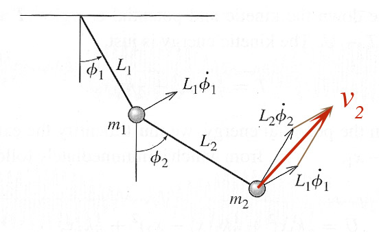
$\phi_1$ - angle away from vertical of the first particle.
$\phi_2$ - angle away from vertical of the second particle relative to
the instantaneous position of particle 1.
To assemble the Lagrangian, we'll need expressions for the kinetic and potential energies of each. These are... $$U_1 = m_1gL_1(1-\cos\phi_1).$$
The height of particle 2 above its resting position is $L_2(1-\cos\phi_2)$ plus the height of particle 1: $$U_2 = m_2g[L_1(1-\cos\phi_1)+L_2(1-\cos\phi_2)].$$
The total potential energy is $$U=(m_1+m_2)gL_1(1-\cos\phi_1)+m_2gL_2(1-\cos\phi_2).$$
The tangential velocity of particle 1 is $L_1\dot{\phi}_1$, so $$T_1=\frac{1}{2}m_1 L_1^2\dot{\phi}_1^2.$$
The two velocity vectors shown beside particle 2 form the sides of a parallelogram, and our desired speed $v_2$ is the diagonal which (squared) leads to $$T_2=\frac{1}{2}m_2(L_1^2\dot{\phi}_1^2 + 2L_1L_2\dot{\phi}_1\dot{\phi}_2\cos(\phi_1-\phi_2) +L_2^2\dot{\phi}_2^2)$$
The total kinetic energy is $$\begineq T&=&\left(\frac{1}{2}m_1 + \frac{1}{2}m_2\right)L_1^2\dot{\phi}_1^2 \\& &+ m_2L_1L_2\dot{\phi}_1\dot{\phi}_2\cos(\phi_1-\phi_2) \\& &+ \frac{1}{2}m_2L_2^2\dot{\phi}_2^2\endeq$$
The resulting Lagrangian is straightforward to write down, but not to solve. For small angles we can get something more tractable. Taylor expanding as necessary, we'll keep no more than 2 orders of terms in any combination of $\phi_1$, $\phi_2$, $\dot{\phi}_1$, and $\dot{\phi}_2$.
In the kinetic energy, we only need to approximate the cosine term as "1", leaving: $$\begineq T&=&\left(\frac{1}{2}m_1 + \frac{1}{2}m_2\right)L_1^2\dot{\phi}_1^2 \\& &+ m_2L_1L_2\dot{\phi}_1\dot{\phi}_2 \\& &+ \frac{1}{2}m_2L_2^2\dot{\phi}_2^2\endeq$$
For small angles, $\cos(\phi) = \sqrt{1-\sin^2\phi} \approx \sqrt{1-\phi^2} \approx 1-\frac{1}{2}\phi^2$. The potential energy simplifies to $$U=\frac{1}{2}(m_1+m_2)gL_1\phi_1^2+\frac{1}{2}m_2gL_2\phi_2^2$$
Now we apply our two Euler-Lagrange equations $$\frac{d}{dt}\frac{\del {\cal L}}{\del \dot{\phi}_1} = \frac{\del {\cal L}}{\del \phi _1} =>$$ $$(m_1 + m_2)L_1^2\ddot{\phi}_1 + m_2L_1L_2\ddot{\phi}_2=-(m_1+m_2)gL_1\phi_1$$
and $$\frac{d}{dt}\frac{\del {\cal L}}{\del \dot{\phi}_2} = \frac{\del {\cal L}}{\del \phi _2} =>$$ $$ m_2L_1L_2\ddot{\phi}_1 + m_2L_2^2\ddot{\phi}_2=-m_2gL_2\phi_2$$
Let's write these as a matrix equation $$\mym{M}\ddot{\myv{\phi}} = -\mym{K}\myv{\phi}$$
The two matrices are: $$\mym{M}=\begincv (m_1+m_2)L_1^2& m_2L_1L_2\\m_2L_1L_2&m_2L_2^2\endcv$$ and $$\mym{K}=\begincv (m_1+m_2)gL_1&0\\0&m_2gL_2\endcv$$
And once again we'll guess complex oscillatory solutions $$\label{thosephis}\myv{\phi}(t) = \begincv \phi_1(t) \\ \phi_2(t)\endcv={\text Re} \[ \begincv a_1\\a_2\endcv e^{i\omega t}\].$$ With this form of the solution, $$\mym M \ddot{ \myv \phi} = -\omega^2 \mym M\myv \phi$$ and the two E-L equations can be written as an eigenvalue equation: $$\[ \mym K -\omega^2\mym M \]\begincv \phi_1(t)\\ \phi_2(t) \endcv =\[ \mym K -\omega^2\mym M \]\begincv a_1\\ a_2 \endcv e^{-i\omega t} = 0. $$
Equal lengths and masses
Setting $m_1=m_2=m$ and $L_1=L_2=L$ we can proceed as before to solve eigenvalue equations. Using the frequency of a single pendulum $\omega_0=(g/L)^{1/2}$to re-write $g=L\omega_0^2$: $$\mym{M}=mL^2\begincv 2& 1\\1&1\endcv$$ and $$\mym{K}=mL^2\begincv 2\omega_0^2&0\\0&\omega_0^2\endcv$$
The eigenvalue equation to solve is $$\label{evalue}(\mym{K}-\omega^2\mym{M})\myv a=mL^2\begincv 2\omega_0^2-2\omega^2&-\omega^2\\-\omega^2 & \omega_0^2-\omega^2\endcv\begincv a_1\\ a_2\endcv=0$$
Setting the determinant of the 2 x 2 matrix to 0 gives us this equation, quadratic in $\omega^2$:, $$2(\omega_0^2-\omega^2)^2-\omega^4 = \omega^4-4\omega_0^2\omega^2+2\omega_0^4 = 0$$
The solutions are: $$\omega_1^2=(2-\sqrt{2})\omega_0^2\ ;\ \ \omega_2^2 = (2+\sqrt{2})\omega_0^2 .$$
Substituting $\omega=\omega_1$ into the eigenvalue equation \eqref{evalue}: $$mL^2\omega_0^2(\sqrt{2}-1)\begincv 2 & -\sqrt{2}\\-\sqrt{2}&1\endcv\begincv a_1\\a_2\endcv=0,$$
To get the ratio of $a_1$ to $a_2$ the constants in the front of the matrix can be ignored, and we just expand the matrix times $\myv a$ to get the two equations: $$2a_1 -\sqrt 2 a_2=0$$ $$-\sqrt 2 a_1 +a_2=0$$
Which implies that $a_2=\sqrt 2 a_1$, or substituting back into \eqref{thosephis} the full time-dependent solution is: $$\myv{\phi}(t) = A_1\begincv 1 \\ \sqrt{2}\endcv\cos(\omega_1t-\delta_1)$$
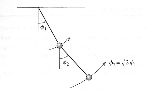 The two particles are in phase, but the bottom one has a larger amplitude.
For the second mode, we get: $$(\mym{K}-\omega^2\mym{M})\myv a=mL^2\omega_0^2(\sqrt{2}+1)\begincv 2&\sqrt{2} \\ \sqrt{2}&1\endcv\begincv a_1\\a_2\endcv=0$$ So the ratios of the amplitudes are $a_2=-\sqrt 2 a_1$.
 In this mode, the particles are exactly $\pi$ radians out of phase. But the ratio of the amplitudes is the same.
Lotsa oscillators
 While we won't go through the procedure again for more than two, you can perhaps see the same general outline for solving systems with more particles and constraints.
Here is the cartoon of the normal modes for three particles coupled by two springs.
Homework
Chapter 11- problems: 17, 18.
11.17 - The normal frequencies:
- $\omega_1^2=\frac 34\omega_0^2$ and you should find that $3a_1=a_2$.
- $\omega_2^2=\frac 32\omega_0^2$ and $3a_1=-a_2$.