Constrained systems
The Lagrangian approach is equivalent to both Newton's equations, and Hamilton's Principle for unconstrained motion, in any coordinate system.
We would like to show that it also works for treating constrained systems.
First, we'll just try out the Lagrangian approach on a constrained system where we can easily calculate what the motion is going to be like using Newtonian mechanics. Do we get the same answer with the Lagrangian approach?
Particle moving up and down a frictionless ramp
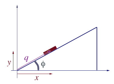 Consider a particle moving up and down the frictionless ramp pictured, tilted at angle $\phi$, subject to gravity.
A constraint
- The particle is moving within the $x,y$ plane. Certainly two coordinates can be used to locate the particle.
- But let's say the particle remains in contact with the ramp:
- Not all positions $(x,y)$ are allowed,
- Only those coordinate pairs are allowed, which have this relation (equation of constraint): $$y/x = \tan (\phi).$$
Newtonian mechanics says
- The gravitational force has a tangential component acting along the ramp: $$F_q=-mg \sin (\phi).$$
- There is also a normal force directed at right angles to the ramp, but it will not contribute to the acceleration of the mass along the ramp (at right angles to the surface of the ramp).
- $\Rightarrow$The equation of motion is: $$m\ddot{q} = -mg\sin(\phi).$$
The Lagrangian approach
- Write down ${\cal L} = T - U$ in terms of some the convenient coordinate $q$ along the ramp:
- Kinetic energy: $$T=\frac{1}{2}m\dot{q}^2.$$
- Write the potential energy, $U=mgy$, in terms of $q$: $$U(q) = mg(q \sin \phi).$$
- The Lagrangian for this constrained system is then $${\cal L} = \frac{1}{2}m\dot{q}^2 - mg \sin (\phi) * q$$
- Write out the Euler-Lagrange equation for coordinate $q$: $$\frac{\del {\cal L}}{\del q} = \frac{d}{dt}\frac{\del {\cal L}}{\del \dot{q}}$$
- Evaluate the derivatives: $$-mg\sin(\phi) = \frac{d}{dt}\left(\frac{1}{2}m*2*\dot{q} \right) = m \ddot{q}.$$
This is indeed the same equation that comes out of a purely Newtonian analysis. So it seems like there might be some hope that this Lagrangian approach works for constrained systems as well as unconstrained systems.
Generalized Coordinates
In the previous example, $q$ is a convenient parameter, which is sufficient (in conjunction with the constraint equation) to fully locate the particle in 2 dimensions.
This is an example of a useful "generalized coordinate". It's often the case that the number of such generalized coordinates needed to uniquely locate the system in space is fewer than the number of particles, $N$, (times) the number of dimensions:
Counting coordinates...
The positions of every particle in a system of $N$ particles can be specified by $N$ 3-d position vectors $\{\myv{r}_1, \myv{r}_2, ... \myv{r}_N\}$.
Or, since there are 3 components to every vector, a total of 3N scalars.
A set of scalars $q_1,....q_n$ make up a set of generalized coordinates if the position vectors can be written as a function of the $q_1,...,q_n$ and time $t$:
$ \myv{r}_\alpha = \myv{r}_\alpha(q_1,...,q_n, t) $ where $[\alpha=1,...,N],$
and each $q_i$ can be written as a function of the $\myv{r}_\alpha$'s and time: $q_i = q_i(\myv{r}_1,...\myv{r}_N, t)$ where $[i=1,...,n].$
Rigid body
 A rigid body is one where the relative positions of all the ($\gg
10^{23}$) particles making up the body are fixed relative to each other.
A rigid body is one where the relative positions of all the ($\gg
10^{23}$) particles making up the body are fixed relative to each other.
We can in principle figure out the position $\myv{r}_\alpha$ of any particle in the football from just:
- the 3 coordinates of the center of mass, and
- 3 more coordinates that specify how the body is oriented.
So, just 6 generalized coordinates suffice to uniquely specify the positions of all the particles in the football.
Pendulum in an accelerated boxcar
Consider a pendulum swinging in a plane (the $x,y$ plane) inside a boxcar, where the boxcar has a constant acceleration $a$.
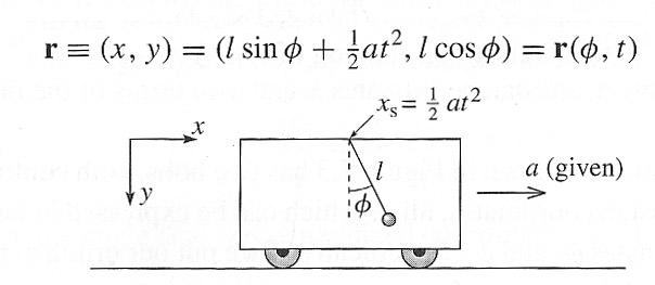
It looks like we can write the position of the pendulum bob in terms of just one parameter $\phi$, the time $t$ and a few constants.
The boxcar is, apparently, a non-inertial reference frame. But it turns out that as long as we write down the kinetic energy and potential energy of the pendulum in an inertial reference frame, the Lagrangian approach will still work to find the equation of motion.
In an inertial frame, the position of the mass on the end of the pendulum in the accelerating boxcar is given by $\myv r(\phi(t),t)=x(\phi(t),t)\uv x+y(\phi(t),t)\uv y$ as in the diagram above.
- Use $U=mgy$ to write $U$ in terms of the single generalized coordinate $\phi(t)$ (and possibly $t$)
Correction! Since $y$ is positive (down), the potential energy is $$U=\color{red}-\color{black}mgy=-mgl\cos\phi$$.
- Take the time derivative of the position vector, $ \dot{\myv r}=(\dot x,\dot y)\equiv(v_x,v_y)$ to get the velocity.
We found $$\dot{\myv r}=\dot x\uv x +\dot y\uv y=(l\cos(\phi)\,\dot\phi+at)\,\uv x -l\sin(\phi)\,\dot\phi\,\uv y)$$
- Calculate $T=\frac 12m v^2=\frac 12m (v_x^2+v_y^2)$.
$$\begineq T =& \frac m2\left[ (l\cos(\phi)\,\dot\phi+at)^2+(l\sin(\phi)\,\dot\phi)^2\right]\\ =&\frac m2\left[\color{blue}l^2\dot{\phi}^2\cos^2(\phi) \color{black}+2atl\dot\phi\cos(\phi)+a^2t^2 +\color{blue}l^2\dot{\phi}^2\sin^2(\phi)\right]\\ =&\frac m2\left[\color{blue}l^2\dot{\phi}^2 \color{black}+2atl\dot\phi\cos(\phi)+a^2t^2\right] \\ \endeq $$
- Set up the Lagrangian for this system, ${\cal L}(\phi(t), \dot\phi(t), t)=T-U$.
$${\cal L} = \frac m2 l^2\dot{\phi}^2 +matl\dot\phi\cos(\phi)+\frac m2a^2t^2\color{red}+\color{black}mgl\cos(\phi).$$
- Calculate both sides of the E-L equation $$\frac{\del {\cal L}}{\del \phi}=
\frac{d}{dt}\left(\frac{\del {\cal L}}{\del \dot{\phi}}\right).$$
$$\begineq \frac{\del {\cal L}}{\del \phi}=& \frac{d}{dt}\left(\frac{\del {\cal L}}{\del \dot{\phi}}\right)\\ matl\dot\phi(-\sin\phi)+mgl(-\sin\phi)=& \frac{d}{dt}\left( l^2\dot\phi+matl\cos\phi \right)\\ \color{blue}-matl\dot\phi\sin\phi \color{black} -mgl\sin\phi=& l^2\ddot\phi+mal\cos\phi + \color{blue}matl(-\sin\phi)\dot\phi\color{black}\\ -mgl\sin\phi=& ml^2\ddot\phi+mal\cos\phi \\ \endeq $$
- Solve for $\ddot\phi(t)$ which should *not* depend explicitly on time. Show that there is an "equilibrium" value of $\phi$, such that $\ddot \phi=0$.
And this equilibrium angle is $\phi_\text{equilibrium}=\arctan(-a/g)$ with the vertical.
Solving for $\ddot \phi$: $$\ddot{\phi}=-\frac {g}{l} \sin\phi-\frac al \cos\phi. $$ At equilibrium $\ddot \phi=0=-\frac{g}{l}\sin\phi_\text{eq}-\frac al\cos\phi_\text{eq}$. This implies that $$\begineq g\sin\phi_\text{eq}=&-a\cos\phi_\text{eq}\\ \frac{\sin\phi_\text{eq}}{\cos\phi_\text{eq}}=&-\frac{a}{g}\\ \tan\phi_\text{eq}=&-\frac{a}{g}\\ \color{red}\phi_\text{eq}=&\color{red}\arctan\left(-\frac ag\right). \endeq$$
-
Make a graph of $\ddot\phi(\phi)$. Set $l$ to some convenient value, like 1. In Desmos, you could code $g$ as 9.8, and then put in a slider for "$a$". Since the pendulum can't go above the ceiling of the boxcar, a natural domain of your graph could be $-\frac{\pi}{2}\lt \phi \lt \frac{\pi}{2}$.
From this graph, is it possible to determine whether the equilibrium position is stable, or unstable? If so, how?
Degrees of freedom
In the ramp example, when the particle slides along the ramp and we vary its $x$-coordinate, the $y$-coordinate is not free to take on any value. It is fully determined if we specify the $x$-coordinate, and are aware of the constraints on the system. We say that there is only one degree of freedom.
Degrees of freedom - The number of coordinates that can be independently varied for small displacements.
 The
double-pendulum system has two degrees of freedom...
The
double-pendulum system has two degrees of freedom...
It seems like, most of the systems we've considered have the following characteristic
Holonomic system
A system in which the number of degrees of freedom $n$ is equal to the number of generalized coordinates $q_1, ..., q_n$ needed to uniquely specify the position of the system.
An exception...
A bowling ball rolling along a line is a holonomic system with 1 degree of freedom. The position of the finger holes is completely determined by the distance along a line that the ball has rolled.
Now consider rolling the ball about on a 2-d surface. If the ball is allowed to roll on a plane, but not 'spin' in place, then it has only two degrees of freedom. But the position of the finger holes still depends on the path taken.
Therefore, more than two coordinates are needed to uniquely specify the position of all the particles in the ball. This is a non-holonomic system.
The result of section [7.4], which we will not go over in detail is to prove that
- for holonomic systems,
- with generalized coordinates $q_1,...q_n$ and
- with potential energy $U(q_1,...q_n, t)$ (that is, conservative non-constraint forces),
that the system will evolve over time according to $$\frac{\del {\cal L}}{\del q_i} = \frac{d}{dt}\frac{\del {\cal L}}{\del \dot{q}_i}$$
Homework
Read: Chapter 7, section 4
Chapter 7, problem 9, 10, 17