Potential boundary conditions, but no charge distribution

We know how to find the field...

From some known charge distribution: $\myv E = \frac{1}{4\pi\epsilon_0}\int\frac{\rho(\myv r')}{\rr^2}\uv \rr\,d\tau'$,
Or from a potential specified everywhere...$\myv E = -\myv \grad V$.

What if we don't have either one of these??

It turns out we can solve a differential equation to find $V$...

In the (hokey) charge on conductors picture, we know the potentials and shapes of the conductors. What we don't know:

How is the charge distributed on the conducting surfaces?
What's the electric potential $V(\myv r)$ between the conductors?

Mathematically, this involves solving...

Laplace's equation

If the region between conductors is empty of charge, then that means at every point in the region... $$\myv{\grad}\cdot \myv E = \rho/\epsilon_0 = 0.$$

But our boundary conditions are in terms of the potentials, not of the fields.

Write this in terms of potentials instead: Substituting $\myv E = -\myv \grad V$ into the equation above... $$\myv{\grad}\cdot\left( -\myv \grad V)\right) = -\grad^2 V = 0.$$ Multiplying both sides by an innoccuous -1, this is Laplace's Equation:

$$\grad^2 V = 0 = \frac{\del^2 V}{\del x^2} + \frac{\del^2 V}{\del y^2} +\frac{\del^2V}{\del z^2}.$$

This is the equation that we need to solve, subject to certain boundary conditions.

The solutions to Laplace's equations are called harmonic functions.

For a function of one variable, the second derivative is a measure of "curvature". To generalize to higher dimensions, $\grad^2 V$ is a measure of the curvature averaged over all directions.

Solutions in one dimension

[The field between two, practically infinite, flat conductors, with no charge between them, with surface normals in the $\uv x$- direction.]

Translational symmetry means that $\myv E = E(x)\uv x$. Show that this leads to... Laplace's equation in one dimension: $$\Rightarrow\frac{d^2V}{dx^2} = 0.$$

The first derivative of a 1-d function is its slope, and the second derivative is the local "curvature" at that point. This equation says that $V$ has zero curvature, that is, solutions are straight lines: $$V=mx + b$$.

A solution that matches the boundary conditions (represented by two blue dots) is shown at right:

Some trivial-sounding characteristics of this solution that are also shared with higher-dimensional solutions:

a minimum or maximum can only occur at the boundary--never in between.
V(x) is everywhere the average value of the function evaluated at points equidistant in $x$. That is: $V(x)=\frac{1}{2}[V(x+R) + V(x-R)]$.

This last statement is the 1-d version of Gauss's harmonic function theorem, which states that $V(x)$ is the average of the values of $V$ on a "sphere" of radius $R$ centered at $x$.

Two dimensions

Now Laplace's equation is $$\frac{\del^2 V}{\del x^2}+\frac{\del^2 V}{\del y^2} = 0$$.

We can think of "V" as representing the height of a landscape as a function of position $x$ (East/West position) and $y$ (North/South position). The "curvature" point of view means that at every position, the landscape is either flat, or the curvature in the $x$- direction is equal and 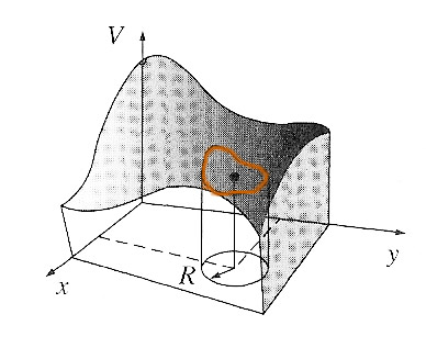opposite of the $y$-curvature:

Example solutions in 2-d, $V(x,y)$

A flat plane should satisfy Laplace's equation: $$V(x,y)=1.$$ It's flat which geometrically means that it has no curvature when moving in the $x$ direction, nor moving in the $y$ direction.

A slightly more interesting example is: $$V(x,y)=x^2 - y^2$$

This defines what is known as a minimal surface.

A soap film suspended from a wire is another example of a physical surface that is a minimal surface.

Again no local minima or maxima are allowed, except at the boundary. For, at a minimum (or a maximum) the curvature in both the $x$- and $y$-directions would have to be the same.

A ping-pong ball placed on a such a surface would have to roll off: it could find no resting place.

The 2-d version of Gauss's harmonic function theorem involves an integral over a circle centered at $(x,y)$: $$V(x,y) = \frac{1}{2\pi R} \oint_{\text{circle}} V dl$$ That is, $V$ is the average value of the $V$ at all the points on a 2-d sphere (a circle) centered at $(x,y)$.

Computer solutions

This is the basis for the method of relaxation: On a computer you can make random guesses at a mesh of points at positions in space. You can find a solution to Laplace's equation by replacing each point by the average of all equidistant points. After enough iterations, the values converge to a solution.

1-d solution in a spreadsheet

Let's actually do this in a spreadsheet...

In 1-d the Laplace equation is $$\frac{d^2V}{dx^2}=0$$ Of course, it's possible to solve Laplace's equation in 1-d exactly. The solution is a straight line, $V(x)=mx+b$, where the constants are set by the boundary conditions.

But instead, I'd like you to use the numerical "method of relaxation" in 1-d to find the solution: Solve this for boundary conditions $V(0)=$20 V and $V(10)=$0 V:

Set up a row of column position labels: 11 column labels representing x=0...10
Set up the next row to represent V(x) set the first column (x=0) to 20 and the last column (x=10) to 0.
Put random numbers in the columns in-between (let's say, between -50 and +100). I did this with this formula in Google Sheets: 150*rand()-50. But then I had to copy my calculated numbers as "values" to keep them from changing with subsequent calculations. The numbers in this row represent some arbitrary 'guess' at the potential, which we will now refine, one iteration (row) at a time.
In the next row down, and all subsequent rows, copy the values for V(x=0) and V(x=10) from the row above.
In betweeen, column $i$ from (1...9) will be calculated by averaging the values for $V_{i-1}$ and $V_{i+1}$ from the row above. Make the spreadsheet do the calculation and eventually copy your formula as needed.

My spreadsheet looks like this initially. I drew the red arrows to show the numbers that are being averaged together from the row above, into one cell in the row below.

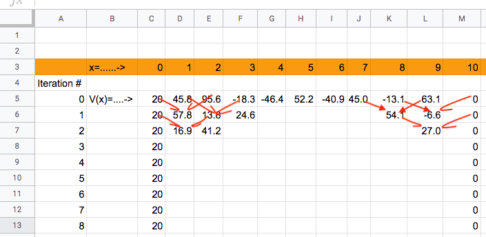
Now, copy/paste to get about 30 rows. Or maybe 60 or 120? See how many iterations you need to go before it looks like the you have a nice monotonic decrease in potential from x=0 to 10...

Three dimensions

It's harder to draw a picture of a field satisfying Laplace's equation in 3 dimensions.

Again, no minima or maxima are allowed except at the boundaries. An interesting consequence of this is that no electrostatic field can hold a charged particle still. (This is too bad if you'd like to confine a plasma, for example..).