Free particle solutions
JoLynne Martinez, Prairie Sky 06

Consider the "Kansas potential":
$$V(x)=0\ \ \ \ \text{for all} \ x.$$
- Sinusoidal "stationary" solutions to the time independent Sch eqtn exist for $E>V$, but they cannot be normalized. (?!)
- Solutions for *any* $E>V$ (Energy is not quantized).
- The stationary states can still be used as basis states.
- Some superpositions of the basis states ("wave packets") *can* be normalized.
- This gets us into the mathematics of Fourier transforms.
Free particle potential
Free particle: $V=0$ everywhere.
Writing the time independent Schrödinger equation out for $\psi(x)$ (instead of $\varphi(x)$): $$\hat H\psi=-\frac{\hbar^2}{2m}\frac{d^2\psi}{dx^2} = E\psi.$$
Re-arrange to get $$ \frac{d^2\psi}{dx^2} = -\frac{2mE}{\hbar^2}\psi \equiv -k^2\psi.$$ Where the new constant $k$ is... $$k\equiv\sqrt{2mE}/\hbar$$
Sketch some solutions for $V(x)=0$ if $E\lt 0$; if $E\gt 0$. Now make $E$ even more $\gt 0$...
The solutions to this second-order differential equation are sinusoids with two free parameters, but there are many ways to write these. We'll use... $$\psi_k(x)=Ae^{ikx}+Be^{-ikx}.$$
Unlike the square well, the boundary conditions (none) allow any value of $k$, and that means any value of $E=\hbar^2 k^2/(2m)$.
Since this Hamiltonian is time-independent, we can add on the time dependence for stationary states $\psi_k$ by multiplying by the factor $\phi(t)=e^{-iEt/\hbar}$ to get the full solution in time and space:
$$\Psi_k(x,t) = Ae^{ik(x-\frac{\hbar k}{2m}t)} + Be^{-ik(x+\frac{\hbar k}{2m}t)}.$$
Two surprises
Our solution... $$\Psi_k(x,t) = Ae^{ik(x-\frac{\hbar k}{2m}t)} + Be^{-ik(x+\frac{\hbar k}{2m}t)},$$
consists of one function of $x+vt$ (and one of $x-vt$).
Consider the function $\varphi_k(x)=Ae^{ikx}$. What happens when we operate on this with the momentum operator $\hat p$?
$$\begineq
\hat p\varphi_k(x)&=\left(-i\hbar\frac d{dx}\right)Ae^{ikx}\\
&=A(-i\hbar)ike^{ikx}\\
&=\hbar k Ae^{ikx}\\
&=\hbar k \varphi_k(x)\\
\endeq$$
Hey, it's an eigenstate of $\hat p$! So we immediately conclude
$$p=\hbar k.$$
This is just a
translation of the function at $t=0$ to the right (left) as time $t$ increases.
That is, this solution function is moving right (or left) with the speed:
$$v_{quantum}=\frac{\hbar |k|}{2m} = \sqrt{\frac{E}{2m}}.$$
Now, a classical particle with energy $E=\frac{1}{2}mv^2$ would be moving with speed: $$v_{classical}=\sqrt{\frac{2E}{m}}=2v_{quantum}.$$
So, they're not the same???
The second surprising thing happens when we try to normalize a solution, say, for example: $$\Psi_k(x,t)=Ae^{i(kx-\frac{\hbar k^2}{2m}t)}.$$
Problem: Calculate $\Psi^*\Psi$ and show that this solution can not be normalized.
So...
- There are "stationary states" (eigenstates) of this time-independent Sch equation,
- Instead of a discrete energy spectrum, any (positive) energy may occur.
- But these solutions are not normalizable--So a particle cannot be in just one stationary state (so it cannot have a unique energy).
- However, as we shall see, a wave packet can be constructed by summing a variety of frequencies. And the wave packet *is normalizable*.
Mathematically, this does not change the fact that we can still write a general solution to the time-independent equation as a super-position of the separable solutions $e^{ikx}$. The only thing is, because any $E$ (and thus any $k$) is allowed, we write an integral instead of a sum over the separable solutions: $$\Psi(x,t)=\frac 1{\sqrt{2\pi}}\int_{-\infty}^{+\infty}\phi(k)e^{i\left(kx-\frac{\hbar k^2}{2m}t\right)}\,dk\label{full}$$
Compare this to what we wrote in the case of the square well case (discrete: only certain values for $n$) $$\Psi(x,t)=\sum_n c_n \psi_n(x)e^{-i\frac{E_n}{\hbar}t}$$
- We use a $k$ instead of $n$ to index the stationary states. It's a non-discrete, real number.
- $e^{ikx}/\sqrt{2\pi}\equiv\psi_k(x)$ is a stationary solution. But it's a non-normalizable wave train!
- $e^{-iEt/\hbar}$ is the time dependence of a single stationary state in both cases,
- $\phi(k)\,dk$ plays the role of a weighting factor, like $c_n$.
Finding $\phi(k)$
Our typical situation in QM is that we somehow prepare a state, say $\Psi(x,0)$ at time $t=0$. In order to see how it evolves with time, we need to write out the state as a superposition of stationary states, because we know how each stationary state evolves in time: $$\Psi(x,0)=\frac{1}{\sqrt{2\pi}}\int_{-\infty}^{+\infty}\phi(k)e^{ikx}\,dk,$$ So, we need to find some way of finding $\phi(k)$.
Remember how we found the amplitudes when we had discrete solutions by "dotting the vector into a basis vector"? $$c_n= \innerp{n}{f(x)}=\int_{-\infty}^{+\infty}\psi^*_n f(x)\,dx$$
Let our stationary (but un-normalizable) solution $e^{ikx}/\sqrt{2\pi}\equiv \ket k$ play the role of the discrete stationary solutions for a well $\psi_n \equiv \ket n$, then our dot product rule for finding the amplitudes in this continuous case would take the form of... $$\begineq \phi(k)=\innerp{ k }{ \Psi(x,0)} &=\int_{-\infty}^{+\infty} \frac{e^{-ikx}}{\sqrt{2\pi}} \Psi(x,0)\,dx\\ &=\frac{1}{\sqrt{2\pi}}\int_{-\infty}^{+\infty} \Psi(x,0)e^{-ikx}\,dx\\ \endeq$$
This is in fact the answer to the question of "How to find $\phi(k)$", and the content of Plancherel's theorem. This result has a name in the field of fourier analysis:
$$F(k)= \frac{1}{\sqrt{2\pi}} \int_{-\infty}^{+\infty} f(x)e^{-ikx}\,dx$$ is called the Fourier transform of $f(x)$.
$$f(x)= \frac{1}{\sqrt{2\pi}} \int_{-\infty}^{+\infty} F(k)e^{ikx}\,dk$$ is called the inverse Fourier transform of $F(k)$.
Example:
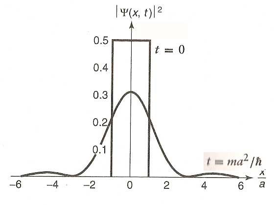
$$\Psi(x,0)=\left\{\begin{array}{cl} A & -a \lt x \lt a\\
0 & \text{ elsewhere}\end{array}\right.$$

...normalization $\Rightarrow A=1/\sqrt{2a}$.
Now, find $\phi(k)$... $$\begineq \phi(k)&=\frac{1}{\sqrt{2\pi}}\int_{-\infty}^{+\infty} \Psi(x,0)e^{-ikx}\,dx\\ &=\frac{1}{\sqrt{2\pi}}\int_{-a}^{+a} \frac{1}{\sqrt{2a}}e^{-ikx}\,dx\\ &=\frac{1}{2\sqrt{\pi a}}\left. \frac{e^{-ikx}}{-ik}\right|_{-a}^{a}\\ &=\frac{1}{2\sqrt{\pi a}} \left(\frac{e^{-ika}-e^{ika}}{-ik}\right)\\ &=\frac{1}{k\sqrt{\pi a}} \left(\frac{e^{ika}-e^{-ika}}{2i}\right)\\ &=\frac{1}{\sqrt{\pi a}} \frac{\sin(ka)}{k}\\ \endeq$$ I've used Euler's theorem that $e^{iw}=\cos w +i\sin w$.
Click to see what happens to $\phi(k)$ as you change $a$, the width of $\Psi(x,0)$:
We shall soon see that $p\propto k$. Does this graph support Heisenberg's uncertainty principle that
$$\sigma_x \sigma_p \geq \frac \hbar{2}?
$$
Now that we have $\phi(k)$, we ought to be able to calculate the wave function at some later time (eq \ref{full}): $$\begineq\Psi(x,t)&=\frac 1{\sqrt{2\pi}}\int_{-\infty}^{+\infty}\phi(k)e^{i\left(kx-\frac{\hbar k^2}{2m}t\right)}\,dk\\ &=\frac 1{\sqrt{2\pi}}\int_{-\infty}^{+\infty} \frac{1}{\sqrt{\pi a}}\frac{\sin(ka)}{k} e^{i\left(kx-\frac{\hbar k^2}{2m}t\right)}\,dk\\ &=\frac 1{\pi\sqrt{2 a}}\int_{-\infty}^{+\infty} \frac{\sin(ka)}{k} e^{i\left(kx-\frac{\hbar k^2}{2m}t\right)}\,dk\\ \endeq$$
Messy, but qualitatively: The stationary states (sine waves) with $k$ (high or low?) are traveling faster. These are the ones that will get out of phase faster .
Here's Griffith's calculation at one time after $t=0$: