Lab 1.1 - Quantum Measurement and Spins

[Adapted from an Oregon State 2010 lab ]

Use the HTML 5 Spins simulator.

In this lab, we'll try to get at...How certain can we be about the probabilities that we're estimating from S-G experiments?

Measure the spin projection $S_z$ along the $z$-axis. When you visit the page it probably looks like this:

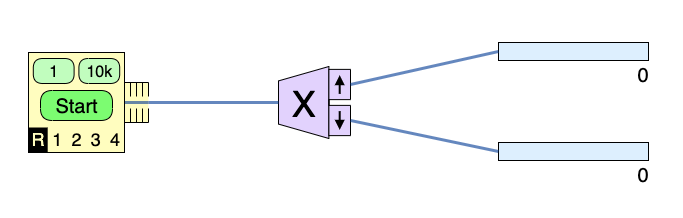
Just click on the analyzer and switch it to "Z".

With the source set to random, "R", each atom emitted has been measured by the Z analyzer as spin up or spin down, denoted by the arrows on the analyzer.

Clicking the 1 on the top of the source sends one atom through the apparatus. Do this repeatedly so you can see the inherent randomness in the measurement process. (Later, you'll want to click 10k to send 10,000 atoms through at a time....) Try running the experiment continuously ("Start"). From the above experiments, and from what we have said in class, you will have surmised that the probability for a spin-up measurement is $P_\uparrow=1/2$, with the probability for spin down being $P_\downarrow=(1-P_\uparrow)=1/2.$ How can we be certain of this? You'll do a series of "experiments" and examine the statistics of the data (see appendix for information about statistics).

You'll need to run multiple trials, each of a fixed number, $N$ of total counts. To get exactly 100 particles through the detector

1. Stop the counting and click Reset so that both counters are at 0.
2. Hit Start.
3. When the sum of the counts in the two detectors gets close to 100, hit Stop.
4. Then click "1" on top of the detector to send one particle at a time through, until the sum of the two detectors is exactly 100.

Now record the number of counts in the spin up detector, $N_\uparrow$. in the first row of the '100' data column table below.

Next you'll repeat this 9 more times to fill up the '100' data column column. (The 10s data column has already been filled up for you.)

Continue, collecting 10 trials of 1000 counts each, then 10 trials of 10,000 counts each. You can hit the 10000 once to get exactly 10,000!

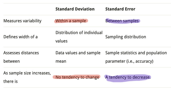
Standard deviation: of the experiment vs of the mean?

Read and refer to Appendix A from the original lab write-up. There is more detail than we will go into, but some of the highlights and necessary details...

• The mean value of a set of $N$ measurements of a random variable $x$ is... $$\overline x = \frac 1N\sum_1^N x_i.$$
• One set of $N$ measurements allows you to calculate one value for the mean, $\overline{x}$. The spread of values of your data "around" the mean is what your experimental standard deviation is measuring. It's written by these authors as "$s$" (which I called "$\sigma$" in our spreadsheet exercise.) They use a definition of $s$ which differs only very slightly from my definition. And the two values converge with very large number of measurements. The "short" way to calculate this standard deviation is $$s=\sqrt{ \frac{1}{N{\color{red}-1}} \left(\sum_1^N(x_i)^2 -N(\overline x)^2\right) }.$$

  
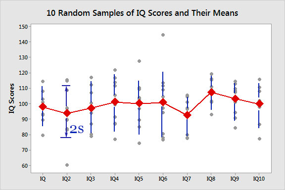
  If the data is distributed according to a "normal" distribution, 68% of measurements of $x$ should fall within the range of values $\overline x - {\color{blue}s}\lt x \lt \overline x +{\color{blue}s}$. So, the vertical length of the error bar for each of the trials in the figure above is ${\color{blue}2s}$, and this varies somewhat from trial to trial.

• But you will likely have noticed that not only $s$ is varying from trial to trial, but the mean ${\color{red}\overline x}$ is also varying! Let's say that we have $M$ trials, and each trial involved $N$ measurements. Apparently here we have $M=10$ trials. Now we can do statistics on the 10 measurements of the mean.
  
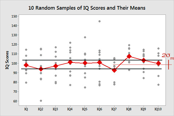
  Assuming again a 'normal distribution', roughly 70% of the measured means should fall within a range of $\pm {\color{red}\sigma_m}$ of the average value of the 10 measurements of the mean! (Here, I have exclude one and a half points above and one and a half below, so as to include $6+1/2+1/2=7$ out of the 10 points in this region beween the black lines.) This is what your author means by the "standard deviation of the mean", $\sigma_m$. And now you can hopefully see how to calculate it, from $M$ different data sets.

  Another term for $\sigma_m$ is the standard error.

• You might expect that your estimate of the mean gets better and better the more measurements you make. So that's what you're testing in this experiment. A summary of the differences (from the website above):
  
  
  So, you'll check your data to see whether...
  • The standard deviation $s$ of the data within any one set of $N$ measurements is approximately constant, whether $N=$10, 100, 1000, or 10000?
  • The standard error of $M$ sets of $N$ sets is going down as $N$ increases?

  Well, actually you'll be measuring the standard error of your probability means. That is ${P_\uparrow} = \overline N_\uparrow/N$, $\sigma P_\uparrow = \sigma\uparrow/N$, and you can calculate $\sigma_m$ from each set of 10 $\overline{P_\uparrow}$ for each $N=$ 10, 100, 1000, 10000.

  Analysis

  Now put the numbers into your calculator or spreadsheet, and find the mean $\overline x$ and standard deviation $s$ of your data, as well as the "standard deviation $\sigma_m$ of the mean". Then calculate the experimental estimate of the probability $P_\uparrow$, its uncertainty, and the relative uncertainty of the mean.

  a. Are you convinced that P  1 2 ? How confident are you? b. How will your results change if you use a larger number for N? c. For any one of your data sets (corresponding to one value for N), perform the statistical calculations by hand and explicitly show them in your lab writeup.