Using Desmos for graphing and data modelling

We'll use some data from an experiment with a radioactive source: A geiger counter was pointed at a sample of radioactive Barium--$Ba^{137}$, to be precise. The geiger count was set up to count the number of decays (clicks) in 30 second intervals.

The experiment started at time=0. In the first 30-second interval (graphed at $t=30$ seconds) there were 130 decays counted. In the second interval (which ended at $t=60$ s), 110 decays were counted. This kept on, for a total of 10 minutes (600 seconds).

You will see that the number of counts decreased as time went on. But not linearly. It looks like the trend was that the number of counts was dropping rapidly at first. But as time went on, the counts were still dropping, but more gradually. This is typical of exponential decay.

Now, follow the screencast yourself, as you do the same operations on a copy of that Desmos file by clicking the image above. Start to make changes to it. Don't worry about messing up that Desmos graph: You will be working with your own copy. (You will need an account on Desmos before you can save your own copy.) You can always get back to the original graph by just clicking the image above, (or re-loading the web page in your browser).

Entering data into a table

DESMOS: entering data and exploring the graph (3 minutes)

Press the + button and add a table.
Each row consists of the $(x,y)$ coordinates of one data point
Points will appear in the graph as you enter them.

Exploring the graph

On a desktop computer you can use these commands to explore or "fly around" the graph. They are similar to what you use to zoom around a Google map.

Mouse scroll wheel forward / backward - zooms in / out
Shift-Mouse drag on the x or y axis - will stretch / shrink just that axis.
Mouse drag - will let you pan: move around to different parts of the graph without zooming.

Axis labels

Click the wrench, near the top right of the graph, to access menus that let you label the axes.

Modelling your data

A model for exponential decay in terms of a half-life is: $$y(t)=p\left(\frac 12\right)^{t/h}$$ What are the meanings of the parameters $p$ and $h$ in this equation?

Perhaps you can see that, when $t=0$, $y(0)=p(1/2)^0=p$. So apparently $p$ would be the number of counts that we would expect *at* $t=0$. This is labelled $p$ to indicate that it's the "principal" or starting amount for the quantity modelled.
Now, notice that, when $t=h$, we have: $$y(t=h)=p\left(\frac 12\right)^{h/h}=p\left(\frac 12\right)^{1}=p\cdot \frac12.$$ The interpretation is that $h$ is the time at which the number of counts has dropped to one half of its initial value. This is the "half-life" of the exponential function.

DESMOS: entering a model equation to fit your data, and adjusting it with sliders. (4 minutes)

Enter the equation for your mathematical model

I'd like to use $t$ to represent the time in my exponential equation. But in Desmos you have to use the variable $x$ to represent your independent variable. So you'll enter the function to use as a model as $y=p*(1/2)^{(x/h)}$:

Press '+' and choose f(x) expression.
Type y=p*(1/2)^(x/h). Actually, you'll have to enter 1/2 [right arrow]) to get the parenthesis around 1/2 to come out right. And use the caret character, ^ to get the exponent as a superscript. Get your function to look like this:
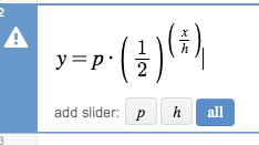
Now, press the all button to add sliders for all of the parameters, $p$ and $h$.
By default, the range on a new slider runs from -10 to 10. But $p$, which represents the number of counts at $x=0$, should probably be close to 150. You can click below where it says "p=1" to set the range on a slider. (See the screencast.) Similarly, a visual estimate of the half-life, $h$, would be the time it takes for the graph to drop from 150 to 75: Somewhere around 180 seconds.
Use the sliders (after you have modified the ranges) to make the graph of your function approximately fit your data.

The best fit

Have DESMOS fit your data for you (5:40 minutes)

Notice that the data table columns are labelled $x_1$ and $y_1$. To get $x_1$ in Desmos, you'll enter x_1 [right arrow].

We'd like our fit to be as "close" to the data points as possible. The distance from each point to the fit function is called its residual (sometimes called "error"). Do this:

In a new function cell type y_1 [right arrow] ~p*(1/2) [right arrow) )^(x_1/h [right arrow] ). Get this to appear:
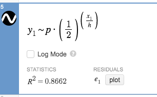
Now press "plot" under the residuals. You should see different colored dots scattered around the $x$-axis.

The residual of the point $(y_1,x_1)$ is the difference in the $y$-coordinate between your model and your point: $e_1 = y(x_1)-y_1(x_1)$.

The "best fit" involves picking parameter values, $p$ and $h$, which minimize some sort of a sum of those residuals. Right now, as you change the parameter sliders, you will see the plots of the residual distances changing and the $R^2$ statistic changing. Actually, minimizing the residuals corresponds to maximizing that $R^2$. Try it!

After you've fiddled with the sliders to get a slightly higher $R^2$, write down the $R^2$ you were able to reach.

Have the computer find the best fit

Desmos has a built-in algorithm for finding the best fit for parameters. To have Desmos do it just give it parameter names that are not associated with sliders:

Edit the cell you just worked on with the subscripts: change the $p$ to $P$ and change $h$ to $H$.

You'll see Desmos' values for the best fit for parameters $P$ and $H$, a graph of the exponential function with those best fit parameters, and the graph of your model with the slider values for the parameters will still be there too.

Probably you will find (check this!) that:

the $R^2$ for Desmos' fit will be somewhat higher than you find while adjusting the sliders, and that
your slider-adjusted parameters were within 10% of Desmos' best fit parameters. Not bad!

I found these values: $P=153.268$ counts, and $H=171.564$ seconds.

Saving your work in Desmos, to hand in via CoCalc

Save your work in Desmos, and hand it in by "embedding" it in a markdown cell. (3:30 minutes)